
The use of population-based disease registries to support ongoing data collection for long-term safety and clinical outcomes is becoming increasingly common. Data collection methods within registries can vary in terms of completeness and quality. This particular example arose from support to a post-registration commitment for marketing authorisation of a paediatric drug and aims to provide some insight to the techniques and strategies used to monitor paediatric development (growth, sexual maturation) and clinical outcomes of varying severity. The challenges of accounting for irregular follow-up and associated biases are illustrated, and potential statistical solutions described. Recommendations for future reporting are presented as part of the conclusions.
Practicalities of working with registry data
Observational data originating from clinical disease registries are utilised in many therapeutic indications as a cost-effective means of collating 'real world' treatment experience on an ongoing basis. Such data can be particularly useful for chronic diseases where progression is likely and longitudinal information is required both for regulatory commitments and for long-term planning. Use of disease registries has increased over recent years, as electronic data capture (EDC) technologies have made data collection a more realistic proposition for clinical sites, which require minimal monitoring and Source Data Verification (SDV) investment.
In contrast to randomized clinical trials, observational studies do not follow strict protocols for the timing of patient visits or clinical evaluations performed at each clinical visit, aiming to reflect the real world clinical setting as much as possible. Consequently, statistical challenges typically relate to patterns of missing data, recording of events/endpoints that are retrospectively reported (recall/selection bias) and events occurring at unobserved, irregular time intervals (interval censoring).
Growth Data: Irregular follow-up and standardization to WHO norms
Chronic diseases evidenced in childhood can severely impact development. Height, weight and BMI can be compared to the World Health Organisation (WHO) centiles. A point estimate (such as the last measured height in Fig 1A) can be plotted against the WHO centiles for a simple graphical display of a snapshot of development in this particular patient population at a specified time point. Graphical techniques such as this can also be used to identify outliers (relative to the expected distribution) and potential data recording errors.
Fig 1A
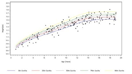
Fig 1B
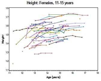
Fig 1C
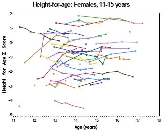
The collection of longitudinal growth data enables an assessment of how the cohort's height and weight compare to international growth norms over the course of the study. In particular, we may wish to test for on-treatment improvement or deterioration in growth. In this setting, growth data is collected at irregular intervals and frequency on each subject (Fig 1B). For each subject, height and BMI are put in the perspective of the height and BMI of healthy children of the same age according to the WHO Growth Standards, using the 'LMS' method (a simplified Box-Cox transformation) to relate the observed data to the Normal [0,1] distribution of the standard population [WHO 2007]. The resulting z-scores express 'height for age' or 'BMI for age' and are used as the endpoint for analysis (Fig 1C).
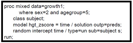
One approach to modelling is to use a random slopes regression, respecting the within-subject correlations in the data (Fig 1D). The fixed effect estimate from this model is the average slope of change in height relative to the international norm. Non-linear extensions to this model should also be considered.
Fig 1D
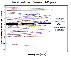
Fig 1E
Dangers lies in interpreting such irregular data, as apparent sub-group trends can result from imbalances in visit frequency of extreme subjects. In addition, there is often interest in charting the progress of subjects in the extreme percentiles, an approach that may be susceptible to 'regression to the mean' bias.
Sexual Maturation Data: Survival data with complex censoring patterns
Sexual maturation was measured using the Tanner Stage, assessing puberty/genital development on a 5 point categorical scale (From Stage 1: pre-pubescent to Stage 5: adult). Irregular follow-up yielded snapshots of a subject's current Tanner Stage. To assess age of onset at a particular Tanner Stage (2 to 5), parametric survival methods were applied, assuming Normality for age of onset. For each patient, age last observed in a given Tanner Stage and first observed in a subsequent stage determined left, right or interval censoring (Fig 2A).
Fig 2A
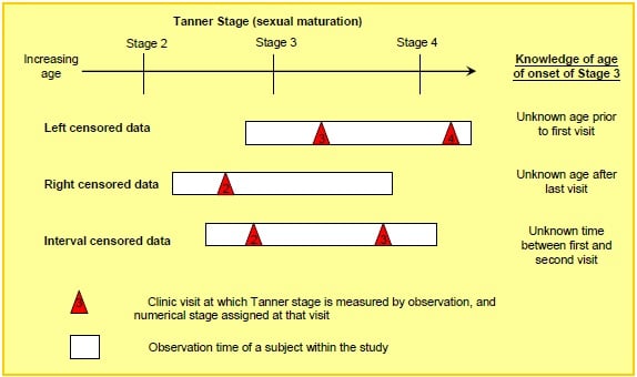
The full transition through the 5 Tanner stages of sexual maturation may take 5 years or more, therefore a cohort study with just a few years observation will have a greatly reduced sample size to assess age of onset of each individual stage (eg. 40 of 209 females in Fig 2B contributed to the estimate for stage 3). The confidence intervals for the median age of onset are therefore wide. However, the appropriately censored estimate makes full use of available data and avoids errors of reporting bias, for example from parental reports, and simplistic approximations such as 'the subject is observed midway between stages'. The estimates were made allowing for the 3 patterns of censoring in Fig 2A using PROC LIFEREG in SAS under a Normal parametric assumption, after examining alternative parametric distributions. These estimates can be compared with the historic 'norms' established by Marshall and Tanner in 1969.
Safety Monitoring: Denominators for person-time
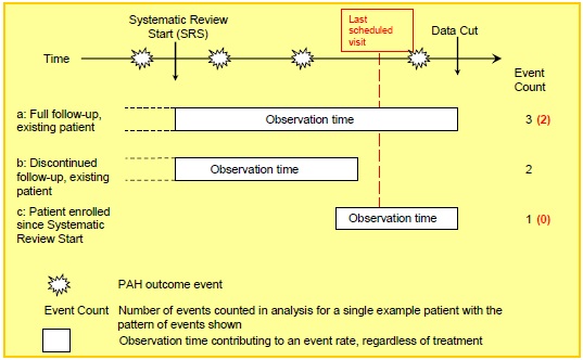
In an observational setting where subjects can enter or exit the population cohort at different times, adverse events can be summarised as event rates, involving the summation of each subject's observation time (Fig 3A). Calculation of observation time can be complicated by considering a variety of possible mechanisms for entry to and exit from the cohort, as well as possible multiple episodes of observation, for example when considering on-treatment exposure.
Fig 3B: Example event rates for graduated outcomes
| Number of Events | Person years | Rate per 100 person years | |
| Increased Liver Enzymes | 5 | 213.8 | 2.3 |
| Hospitalization | 43 | 257.6 | 16.7 |
| Death | 10 | 257.6 | 3.9 |
Under a passive cohort surveillance, the 'severe' outcomes such as hospitalisation and death will be detected at any time until data cut as the outcome is linked to routine medical records systems. 'Mild' outcomes that require a clinic visit will not be detected between the routine visit appointments for registry participants, unless the subject makes an unscheduled clinic visit for other reasons. In Fig 3B, the person years for mild outcomes is adjusted downwards by subtracting observation time after the last recorded visit.
Fig 2B
| Figures are medians and 95% confidence intervals |
Females (Total n=209) |
Males (Total n=167) |
| Stage 2 |
9.5 (8.0 - 11.1) n for stage = 38 |
12.5 (10.6 - 14.4) n for stage = 23 |
| Stage 3 |
13.1 (12.1 - 14.1) n for stage = 40 |
13.0 (12.0 - 14.0) n for stage = 23 |
| Stage 4 |
15.5 (14.3 - 16.7) n for stage = 39 |
16.0 (14.5 - 17.5) n for stage = 24 |
| Stage 5 |
17.2 (15.4 - 19.0) n for stage = 36 |
(no model convergence) n for stage = 14 |
FIGURE 3A
Discussion and Concluding Remarks
We recommend standardization is adopted with full awareness of the nature of the standard. WHO standards comprise a particular ethnic mix, which may not match that of the sample population. Further, comparison with 'healthy' may not reflect the normal expectation of the diseased sample; benchmarking against a wider diseased population may be more relevant.
Graphical visualizations were a valuable tool for data checking during this project, and can be used iteratively to identify outlying subjects and inconsistent longitudinal trends, generating data queries and plot revisions.
In dealing with complex censoring, the fit of any parametric assumption should be checked with diagnostic plots. Optimizing the fit may present a challenge when modelling multiple subgroups, as the same parametric assumption may not apply throughout. Here, 4 stages of onset were modelled for primary and secondary Tanner stages in both males and females.
In addition to denominator adjustment, safety monitoring of milder/less overt outcomes may suffer from bias in the numerator, as the frequency and consistency of reporting may not be a clinical priority in some observational settings.
In conclusion, understanding the mechanism of the registry, alongside a thorough understanding of the disease and population being studied, is crucial in assessing the usefulness and subsequent modelling of registry data.

References
Marshall WA and Tanner JM (1969) Variations in pattern of pubertal changes in girls. ArchDis Child 1969;44:291-303.
Development of a WHO growth reference for school-age children and adolescents. Bulletin of the World Health Organization 2007;85:660-7.
This article was authored by Jeremy Wheeler and Katherine Hutchinson from the Statistical Consultancy team.
Subscribe to the Blog
FOLLOW QUANTICATE ON:


© 2024 Quanticate